Analyzing Bull and Bear Market Cycles in Python
published September 30, 2020
updated July 22, 2022 (updated ML section for appropriate ML variables)
Introduction
This article is the first part of a three-part series of articles. Part 1 (this post) introduces software for analyzing Bull and Bear market conditions in the Python computer language. Ultimately the objective is to build a machine-learning algorithm to predict “Bull” upward trending and “Bear” downward trending market conditions. Creating the market prediction algorithm will employ a standard data science process described in Part 2. Part 2 explores and analyses additional data sources for use in the prediction model. In part 3, the machine learning algorithm is developed and backtested.
Bull and Bear market conditions apply to stock markets such as the S&P 500 or NASDAQ. In summary, the market will be in one of the two conditions. A market with upward trending prices is referred to as a “Bull” market. Typically, a Bull market lasts for an extended period, often years. However, the market can switch to a downward trending market with typical periods ranging from as short as a month to over a year and termed a “Bear” market condition.
Understanding and analyzing market cycles helps investors gain insight into familiar patterns, market conditions, influences on the market, and helps investors to plan investment strategies. In this article, two software tools are introduced for analyzing market cycles in the Python computer language. The fmcycles() function receives as input stock market data, such as S&P 500 daily close price, then retroactively analyzes it and marks the corresponding market dates as corresponding to Bull or Bear market conditions. Also, machine learning features, variables useful for prediction, are derived from the market cycle analysis. The second tool introduced in this article is the fmplot() function for plotting and quickly visualizing stock market data and market cycles.
This article’s content is listed below, including links to the software, several examples, and a summary of machine learning variables generated by the tools. Following the Summary and Conclusions, there are additional references about bear markets that provide further insights.
- Github Links
- Initialization and Data Import
- Analyze Save and Load Market Cycles
- Market Cycle Summary
- Market Cycle Visualization
- Recessions: Annotations and Fill-Between
- Subplots with MktCycle and Line Plots
- Zoom In
- Machine Learning Variables
- Summary and Conclusions
- Market References
Github Links
The programs and corresponding Jupyter nobebook are available as open source via Github at the following links
Initialization and Data Import
The python code for the examples below is contained in the “Market Cycle Notebook” (link above) and available for download on Github.
As with a typical data analysis, we begin by importing packages and modules. Since fmcycle.py and fmplot.py are not yet available within a Python package, it is required to download them and put them into a directory contained in the PYTHONPATH. Downloading the modules into the Jupyter or Python working directory is typically the most straightforward approach.
import pandas as pd
import numpy as np
import matplotlib.pyplot as plt
from datetime import datetime as dt
from datetime import timedelta as td
%run fmplot
%run fmcycle
Next, we import the S&P500 data by downloading the symbol “^GSPC” from Yahoo finance and save it in the “data” directory (./data relative to the python working directory). For this exercise, the market data begins on 1950-01-03 and ends on 2020-08-24.
# Read in S&P 500 Data
dfsp500 = pd.read_csv('./data/GSPC_1950-1-3_to_2020-8-24.csv',index_col=0,parse_dates=True)
display(dfsp500.head(2))
display(dfsp500.tail(2))
            Close	 High  	Low	 Open	 Volume	 Adj Close
Date
1950-01-03	16.66	16.66	16.66	16.66	1260000.0	NaN
1950-01-04	16.85	16.85	16.85	16.85	1890000.0	NaN

            Close	  High     Low     Open      Volume	    Adj Close
Date
2020-08-21	3397.16	3399.96	3379.31	3386.01	3.705420e+09	3397.16
2020-08-24	3431.28	3432.09	3413.12	3418.09	3.728690e+09	3431.28
Analyze, Save, and Load the Market Cycles
The fmcycle.py module contains the fmcycles() function and it receives as input the dfsp500 dataframe. When compute = 1 the market data is analyzed and the function returns the detailed (“daily”) market cycle dataframe dfmc and summary market cycle dataframe dfmcsummary. Each dataframe is automatically saved to a csv file. If compute = 0 then fmcycles() expects to receive filenames to import the detailed and summary market cycle datafames and in this case does not analyze the input dataframe.
The three key parameters used for analyzing the daily market data are mcdown_p, mcup_p, and variable, defined as follows:
- mcdown_p = the percent decline from market high determining a Bear market condition, default = 0.20.
- mcup_p = the percent increase from market low determining a Bull market, default = 0.205.
- variable = the name of the variable contained in the input data frame, df, to analyze, by default = Close
It is possible to set mcdown_p and mcup_p to other cycles, such as 10% corrections, rather than the 20% Bull and Bear conditions. Furthermore, it is also entirely possible to analyze the up and down cyclic performance of any security in this manner other than the ^GSPC. For long term evaluation of an Equity, instead of a market index, the correct variable for analysis will be Adj Close.
f_dfmc="./data/GSPC_dfmc2020.5_1950_2020-8-24.csv"
f_dfmcs="./data/GSPC_dfmcs2020.5_1950_2020-8-24.csv"

compute=0
mcycledown=20
mcycleup=20.5

dfmc,dfmcsummary=fmcycles(df=dfsp500,symbol='GSPC',compute=compute, mc_filename=f_dfmc, mcs_filename=f_dfmcs, mcdown_p=mcycledown,mcup_p=mcycleup,savedir="./data"
Market Cycle Summary
Below, is displayed the dfmcsummary dataframe, which contains a summary of the market cycles. We will explore the detailed market cycles in the dfmc dataframe using the fmplot() function below. The dfmcsummary summary is in agreement with published S&P500 Bull and Bear markets. For example, compare to the the Seeking Alpha article, which contains a listing of historical Bull and Bear market S&P500 markets.
display(dfmcsummary)
   index      mkt	    startTime	   endTime	startPrice	endPrice	    mcnr
  1950-01-03 	 1.0	 1950-01-03	1956-08-02	16.660000	  49.639999	   1.979592
  1956-08-02	-1.0   1956-08-02	1957-10-22	49.639999	  38.980000	  -0.214746
  1957-10-22	 1.0	 1957-10-22	1961-12-12	38.980000	  72.639999	   0.863520
  1961-12-12	-1.0	 1961-12-12	1962-06-26	72.639999	  52.320000	  -0.279736
  1962-06-26	 1.0	 1962-06-26	1966-02-09	52.320000	  94.059998	   0.797783
  1966-02-09	-1.0	 1966-02-09	1966-10-07	94.059998	  73.199997	  -0.221773
  1966-10-07	 1.0	 1966-10-07	1968-11-29	73.199997	  108.370003	 0.480465
  1968-11-29	-1.0	 1968-11-29	1970-05-26	108.370003	69.290001	  -0.360616
  1970-05-26	 1.0	 1970-05-26	1973-01-11	69.290001	  120.239998 	 0.735315
  1973-01-11	-1.0	 1973-01-11	1974-10-03	120.239998	62.279999	  -0.482036
  1974-10-03	 1.0	 1974-10-03	1980-11-28	62.279999	  140.520004	 1.256262
  1980-11-28	-1.0	 1980-11-28	1982-08-12	140.520004	102.419998  -0.271136
  1982-08-12	 1.0	 1982-08-12	1987-08-25	102.419998	336.769989	 2.288127
  1987-08-25	-1.0	 1987-08-25	1987-12-04	336.769989	223.919998	-0.335095
  1987-12-04	 1.0	 1987-12-04	2000-03-24	223.919998	1527.459961	 5.821454
  2000-03-24	-1.0	 2000-03-24	2001-09-21	1527.459961	965.799988	-0.367708
  2001-09-21	 1.0	 2001-09-21	2002-01-04	965.799988	1172.510010	 0.214030
  2002-01-04	-1.0	 2002-01-04	2002-07-23	1172.510010	797.700012	-0.319665
  2002-07-23	 1.0	 2002-07-23	2007-10-09	797.700012	1565.150024	 0.962078
  2007-10-09	-1.0	 2007-10-09	2008-11-20	1565.150024	752.440002	-0.519254
  2008-11-20	 1.0	 2008-11-20	2009-01-06	752.440002	934.700012	 0.242225
  2009-01-06	-1.0	 2009-01-06	2009-03-09	934.700012	676.530029	-0.276206
  2009-03-09	 1.0	 2009-03-09	2020-02-19	676.530029	3386.149902	 4.005173
  2020-02-19	-1.0	 2020-02-19	2020-03-23	3386.149902	2237.399902	-0.339250
  2020-03-23	 1.0	 2020-03-23	NaT	        2237.399902	NaN      	   NaN
For each row we have the start date, end date, start price, and end price of the market variable (close price). The mkt variable indicates if the market is in an up trending (1.0, Bull) condition or in a down trending (-1.0, Bear) condition. The mcnr (market cycle normalized return) variable is the normalized return of the close price, at the end of the cycle, relative to the start date.
Market Cycle Visualization
We plot the detailed market cycle information with fmplot(), which is defined on top of matplotlib. A market cycle plot, plottype =’mktcycle’, designates a stem chart, with the use of colored stems, without a marker (at the top of the stem). We call the fmplot() function with the variable = mcnr. The mcnr variable was derived by fmcycle() and is contained in the detailed market cycle dataframe, dfmc. This variable is set to zero at the beginning of each market cycle. For a Bull market the variable increases (blue), until the last market high, prior to a 20% drop. Similarly, mcnr decreases from zero (red) until the market low prior to the market rising by 20.5% from the low. This is a classic chart used to visualize Bull and Bear markets, for example, look at the Inveso chart for comparison.
There are several additional options used in the example below. Setting titlein = True appends the beginning and ending date of the input dataframe to the title. Most other inputs are easily understood. Documentation for all the input parameters is visible with Jupyter Shit+Tab feature.
title=['Bull and Bear Normalized Returns']
variables=['mcnr']
fmplot(dfmc,variables,titles=title,
          plottypes='mktcycle', stemlw=0.5,legend_fontsize=20,
          titlein=True, titlexy=(0.5,0.95), figsize=(18,10),titledate=True, title_fontsize=20)
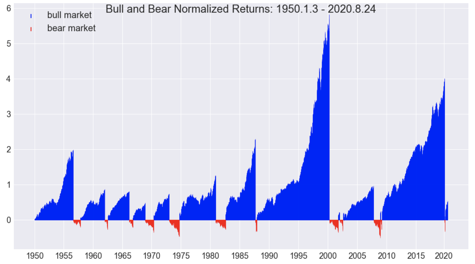
From this graph, it is evident that characterizing the market cycles requires retroactive analysis.
For example, finding a Bear market (down-trending market), assuming we start during Bull upward trending (blue) market condition, starting from earlier dates to later dates, we identify a market-high close price. Initialize the market high to the close price corresponding to the first day of the current market cycle. Then, moving forward day-by-day, we monitor the close price relative to the market high until a new high is found or the market falls by 20% relative to the market high. On the day the market falls by 20% relative to the market high, a Bear market is detected. At this point, we go back (retroactively) and fill in the dates from the high to the present day and mark the days as mkt = -1. The market days before the high are marked as mkt = 1, corresponding to the Bull market. The Bear market starts on the next market day following the previous high. The mcnr variable is set equal to zero at the beginning of the Bear market cycle, and from that point forward to the present, indicates the percent decrease from the market high.
Similarly, once in a Bear market (downward trending market), a Bull market is detected when the market increases by greater than 20% relative to the market low. Once the market has increased by 20% from the market low, we go back (retroactively) and fill in the dates from the market low to the present day and mark the days as mkt = 1. The market days before the market low, from the previous market high, are marked as mkt = -1, corresponding to the Bull market. The mcnr variable is set equal to zero at the beginning of the Bull market cycle, and from that point forward to the present, indicates the percent increase from the market low.
Recessions: Annotations and Fill-Between
It is useful to add additional information to the plot, especially to generate plots for documentation and presentations and for observing insights.
A typical addition is to show recessions. fmplot.py contains the get_recessions() function, which returns a list of recessions in the form of tuples (start date, end date). These are graphed using the fb (fill between) option.
Below, we create a list of text annotations with descriptive titles for the Bull and Bear cycles, and recessions. The list elements include a tuple with the corresponding x and y coordinate, corresponding to where the annotation will be placed on the graph, and a text string. The text string may contain a “\n” character to designate a line return.
# Recession Data
# get recessions and put in dataframe to make it look pretty

recessions = get_recessions()

# Bear Market and Recession Annotations

# Bear Market Annotations
bearannotations=[]
bearannotations.append((dt.datetime(1956,1,1),-1.1,'1956-57\nRed\nScare'))
bearannotations.append((dt.datetime(1961,1,1),-1.3,'1961-62\nSteel &\nTech\nCrash'))
bearannotations.append((dt.datetime(1965,4,1),-1.1,'1966\nCredit\nCrunch'))
bearannotations.append((dt.datetime(1969,4,1),-1.3,'1968-70\nDouble\nBottom\nBear'))
bearannotations.append((dt.datetime(1974,1,1),-1.1,'1973-74\nGolden\nBear'))
bearannotations.append((dt.datetime(1981,1,1),-1.1,'1980-82\nVolker\nBear'))
bearannotations.append((dt.datetime(1987,1,1),-1.1,'1987 Oct\nBlack\nMonday'))
bearannotations.append((dt.datetime(2000,1,1),-1.1,'2000-02\nDot Com\nBubble'))
bearannotations.append((dt.datetime(2007,1,1),-1.2,'2007-09\nFinancial\nCrisis'))
bearannotations.append((dt.datetime(2019,1,1),-1.1,'2020\nCOVID\nBear'))


# Recession Annotations
recessionannotations=[]
recessionannotations.append((dt.datetime(1951,1,1),2.8,'1953-54\nPost\nKorean\nWar\nRecession','k'))
recessionannotations.append((dt.datetime(1956,1,1),3.8,'1957-58\nEisenhower\nRecession','k'))
recessionannotations.append((dt.datetime(1959,1,1),2.5,'1960-61\nRolling\nAdjustment\nRecession','k'))
recessionannotations.append((dt.datetime(1969,1,1),3.2,'1969-70\nNixon\nRecession','k'))
recessionannotations.append((dt.datetime(1973,1,1),2,'1973-75\nOil\nCrisis\nRecession','k'))
recessionannotations.append((dt.datetime(1978,1,1),3.8,'1980\nEnergy\nCrisis\nRecession','k'))
recessionannotations.append((dt.datetime(1981,1,1),2.5,'1981-82\nIran\nEnergy\nCrisis\nRecession','k'))
recessionannotations.append((dt.datetime(1990,1,1),2.8,'1990-91\nGulf\nWar\nRecession','k'))
recessionannotations.append((dt.datetime(2001,1,1),2.8,'2001\n9/11\nRecession','k'))
recessionannotations.append((dt.datetime(2007,1,1),2.8,'2007-09\nThe\nGreat\nRecession','k'))
recessionannotations.append((dt.datetime(2018,1,1),4.2,'2020\nCOVID-19\nRecession','k'))
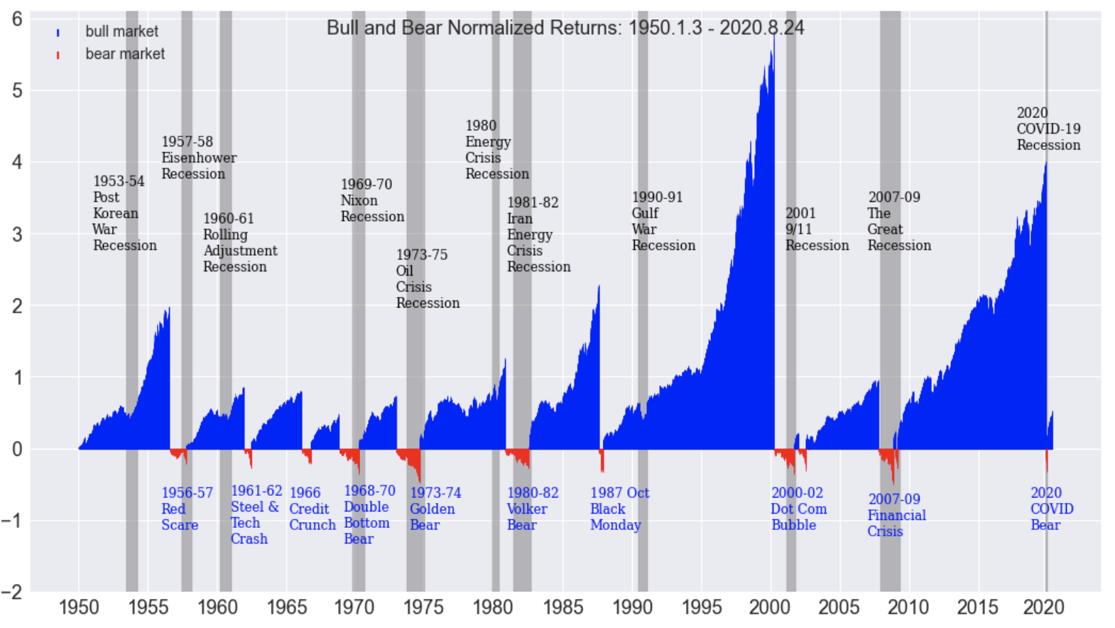
The fmplot() function with fb and annotation options generates the classic Bear and Bull market cycle chart, including a display of recessions and descriptive text.
title=['Bull and Bear Normalized Returns']
variables=['mcnr']
fmplot(dfmc,variables,titles=title,fb=recessions,
          plottypes=['mktcycle'], stemlw=0.5, ylims=(-2,6.1), legend_fontsize=14,
          titlein=False, figsize=(18,10),titledate=True, title_fontsize=18,
          annotations=[bearannotations + recessionannotations])

Several insights result from this graph. Our objective here is not to deep dive into classic market analysis, but especially to make observations that will aid in designing a machine learning model.
- The first most apparent observation is the cyclic behavior of the market. It tends to rise, upward trend line (blue) then goes into a downward trend (red), followed by a repetition of the cycle.
- The upward trend’s length typically occurs for several years, wherein a growing market is the normal situation, but is interrupted by shorter length downward trends or crashes.
- Recessions can occur without causing a market crash. For example, the Gulf War Recession or the post-Korean war recession occurred during Bull markets. Recessions tend to be reactionary to the market, rather than a leading indicator of the market. Often there are market crashes without recessions, and sometimes a recession follows a market crash.
- We learn that often outside forces are the instigators of crashes. A case in point is the 2020 COVID Pandemic. The pandemic crisis had nothing to do with financial markets, but the effect due to social distancing strongly impacted the workforce and business operations across most industries.
- In some cases, the same trends that are driving the market up are the ones that bring the market down. Such a case is the 2007 - 2009 Financial Crisis, where the U.S. housing market, sub-prime mortgage investments, drove the market up and then brought the market down with the collapse of the U.S. housing market.
- In many cases, assets are overvalued and are termed asset bubbles. In such cases, certain metrics, for example, price-to-earnings ratio, increase significantly above historical levels leading to straightforward prediction. A case in point is the DoT Com Bubble, which led to unjustified multi-billion dollar valuations as companies went public. Looking at Figure 3, we observe it took from 2000 to late 2007 to regain the lost market value from the Dot Com Bubble.
- The 1987 Black Monday Bear is a result of several outside influences including computerized trading, fears of the devaluation of the dollar, and military tensions with Iraq.
- The 1980-82 Volker Bear is attributed to the Fed raising interest rates in order to slow inflation, but then making it difficult to borrow money contributing to a high employment rate and a market slow down.
From these observations, it is evident that outside factors have a strong influence on the market. In some cases, market downturns are due to world events such as military conflicts, world politics, and worldwide pandemics. In some cases new technologies such as computerized trading react quickly to cause a stock sell off with devastating effect. In other cases monetary decisions designed to be helpful have harmful side effects. To some degree, following each market crash new policies, practices, and corrections are adopted to prevent future crashes.
From all these observations, there are at least two general points for developing a market cycle prediction model.
- a model will likely have to learn quickly as a new market situation develops.
- additional data sources that capture the effects of external forces should be useful for predicting market downturns. We will explore additional data sources in part 2 of this series.
Subplots with MktCycle and Line Plots
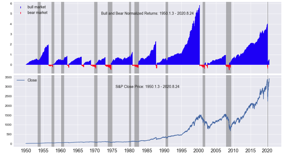
When analyzing variables and trends, it is useful to compare multiple market variables. For example, it is beneficial to examine the mcnr and compare it to the close price. Here we provide fmplot() a list of variables to be plotted along with a list of plot types. We also set hspace indicating a small amount of space between subplots, and set sharex = True for sharing the x-axis for all subplots. More details for these features are available by examining the fmplot() “docstrings” with the Jupyter shift+Tab feature.
title=['Bull and Bear Normalized Returns', 'Close Price']
variables=['mcnr','Close']
fmplot(dfmc,variables,titles=title,stemlw=2,fb=recessions,
          plottypes=['mktcycle','line'],legend_fontsize=14,llocs=['upper left','best'],
          xtick_labelsize=18, hspace=0.025, sharex=True,titlein=True, figsize=(18,10),titledate=True)
Zoom In
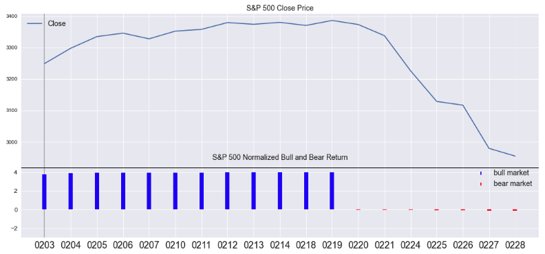
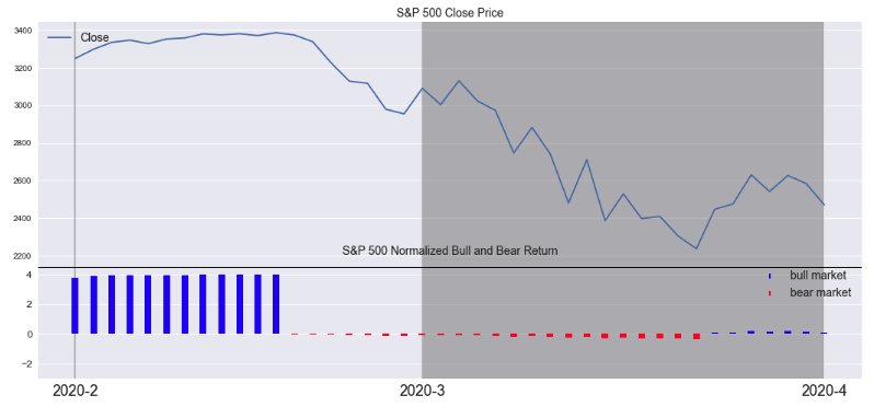
The previous graph displays the entire length of the dataframe from the start date in 1950 to the end date in 2020. It is useful to zoom in and examine narrow ranges of time. Below we zoom into a one-month interval from February 1, 2020, to March 1, 2020 (Figure 4a). The top graph plots Close as a line graph and the bottom subplot graphs mcnr as mktcyle plot. Here we can see the first day of the COVID Bear beginning on Thursday, February 20. We also can observe the rapid market crash ensuing after February 20. The market was up 400% relative to the start of the Bull on March 9, 2009. In the next graph (Figure 4b), we observe the entire Bear market cycle along with the close price by setting dates between February 1, 2020, and April 1, 2020.
figsize=(18,8)
startdate=dt.datetime(2020,2,1)
enddate=dt.datetime(2020,3,1)

titles=['S&P 500 Close Price','S&P 500 Normalized Bull and Bear Return']
variables=['Close','mcnr']
fmplot(dfmc,variables,startdate=startdate,enddate=enddate,legend_fontsize=14,
               plottypes=['line','mktcycle'],stemlw=8,llocs=['upper left','upper right'],
               figsize=figsize,fb=recessions,sharex=True, hspace=0,ylims=['',(-3,5)],xtick_labelsize=18,
               titles=titles,titlexy=[(0.5,0.9),(0.5,0.8)],height_ratios=[2,1],hlines =['',4.5])
Machine Learning Variables
Several variables generated by fmcycle() are useful for creating a machine learning model of the market cycles. It is essential to understand which variables are appropriate for machine learning and which ones are not.
It is tempting to employ mkt variable as the target variable (dependent variable) in the training of the machine learning model. That is, a machine learning algorithm is trained to predict mkt. If a machine perfectly predicts this variable, it amounts to trading only when the market is in an upwardly trending condition (Bull market), and for example, when investing in an S&P500 index fund, results in very significant gains. Such a situation would result in “beating the market.” However, it should be remembered that the mkt signal is determined retroactively so its use as a target variable will inadvertently result in leakage of truth into the training algorithm.
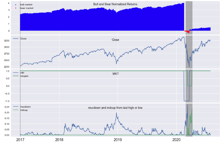
Close, mucdown, mdcup, and mcupm are useful as machine learning features, meaning predictor variables, after proper normalization. These signals are described as follows.
- Close - this variable is the daily market close price and will need to be properly normalized for use as a machine learning feature variable.
- mcupm - This signal is generated by fmcycles() and marks the point in time when the market is in an up or down condition, without retroactive analysis. This signal is not perfectly aligned with mkt as seen in the graph. For example, the market is in a Bull upward trend condition, and a Bear market is not yet detected, so mcupm lags mkt.
- mucdown - This signal is generated by fmcycles(). When in a Bull market condition, mucdown is the percent down from the previously detected market high.
- mdcup - This signal is generated by fmcycles(). When in a Bear market condition, mdcup is the percent up form the previously detected low.
Some variables should not be used for machine learning. The mcnr variable, as described above, is derived by retroactively identifying the market condition. It must not be used for prediction, or “leakage” will occur. Leakage is when the dependent variable leaks back into the machine learning features. In such a case, the machine learning algorithm will unfairly learn and appear to work very well during the training phase, but it will usually perform less effectively in the real world prediction phase due to poor generalization.
startdate=dt.datetime(2017,2,1)
enddate=dt.datetime(2020,8,1)


title=['Bull and Bear Normalized Returns', 'Close',' MKT', 'mucdown and mdcup from last high or low']
variables=['mcnr','Close','mkt',['mucdown','mdcup']]
fmplot(dfmc,variables,titles=title,startdate=startdate,enddate=enddate,stemlw=2,fb=recessions,
          plottypes=['mktcycle','line','line','line'],xtick_labelsize=18,
          hspace=0.025,sharex=True,titlein=True, titlexy=[(0.5,0.85),'','',''],
          figsize=(18,12))
Summary and Conclusions
In summary, this post is the first in a three-part series. This article (Part 1) contributes two functions for analyzing the market. The fmcycle() function analyzes close price information to identify Bull and Bear market conditions, while fmplot() offers an easy to use plotting tool necessary for visualizing time series based stock market data. The ultimate objective of this blog series is to develop a machine learning model for the prediction of Bull and Bear market conditions. Part 2 explores and analyzes additional data sources for use by the predictive model, and Part 3 develops the predictive model and tests the resulting financial performance with backtesting.
The result of applying fmcycle() to the S&P 500 data downloaded from Yahoo Finance is the generation of the detailed and summary market cycle dataframes, dfmc and dfmcsummary. The summary dataframe contains start and end Bull and Bear market cycles, including mcnr (Market Cycle Normalized Return). The results for start, end, and normalized return for each Bear and Bull market cycle match those reported elsewhere back to 1950. The detailed dataframe contains the mkt variable for each trading day marked as either +1 or -1, indicating the market is in a Bull (upward trend) condition or Bear (downward trend) condition. The detailed data frame also contains the daily mcnr relative to the start of the current cycle.
Essential insights are gained by plotting the detailed market cycle dataframe’s (dfmc), mcnr variable with fmplot() and observing the market cycle behavior. Numerous insights are observed from the fully annotated chart of Bull & Bear Markets and recessions, which are useful for understanding market behavior and thus building a market cycle prediction model. Additional insight is learned by zooming into specific dates and comparing the mktcycle plot with line plots of the market close price.
The fmcycles function generates variables that are essential for developing a market cycle prediction model. It is important to note that the mcnr variable and mkt are not appropriate to use as a prediction variable or truth variable, since they are derived retroactively from future dates, and would result in leakage. Additional variables generated by fmcycle() that are useful for machine learning are mucdown, mcdup, and mcupm. These variables will be explored further in Parts 2 and 3 of this article series.
Market References
[1] Asset Bubbles, Investopedia
[2] Invesco, Listing of Bear and Bull Market Cycles , Invesco
[3] Past Recessions, Investopedia
[4] History of Bear Markets since 1929, Fox Business
[5] The Golden Bear, Marotta on Money
[6] The Dot Com Bubble, Marotta on Money
[7] Historic Bear Markets, NBC News